


What Is a Noise Figure? Why an Amplifier Adds Noise
The noise figure (NF) is the core figure for the noise performance of an optical amplifier: it describes how much the signal-to-noise ratio degrades as the signal passes through. Understanding its physical meaning, its quantum limit and the differences between amplifier types matters for system design and device selection. This article covers the concept, the formulas, the classification and the applications of the noise figure.
Table of contents
- 1. What is a noise figure? Getting the core concept straight
- 2. Working principle: where the noise of an amplifier comes from
- 3. Key parameters: reading the specifications of the noise figure
- 4. Main types: what kinds of noise figure are there
- 5. Applications: where does the noise figure matter
- 6. Common misconceptions: points easily confused
1. Core concept: what is a noise figure?
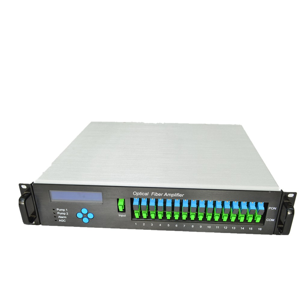
The noise figure (NF) is the core measure of how much extra noise an optical amplifier introduces while amplifying. In simple terms it describes how much the signal-to-noise ratio (SNR) degrades as the signal passes through: the lower the noise figure, the better the noise performance.
The definition is the ratio of the SNR at the input to the SNR at the output, usually expressed in dB. An ideal noiseless amplifier would amplify the signal and the input noise by the same factor, leaving the SNR unchanged, so its noise figure would be 0 dB. Every real amplifier adds noise, however, so the noise figure is always above 0 dB. The noise figure is one of the most important specifications of an optical amplifier; for a preamplifier and for long-haul systems it often matters more than gain.
The noise figure determines how much signal-to-noise ratio survives the amplifier, and with it the number of stages a link can carry, the receiver sensitivity and the ultimate reach. In long-haul communication and weak-signal detection it is often worth confirming before anything else.
One easily overlooked property of the noise figure is that it does not depend on the signal power, only on the amplifier itself. However strong the input, the amplifier takes the same fixed cut out of the signal-to-noise ratio — which is why a link budget can simply plug the noise figure of each stage into the formula and accumulate them.
2. Working principle: where the noise of an amplifier comes from
To understand the noise figure, it helps to be clear about what noise an amplifier actually adds. In short, while amplifying the signal it also amplifies the spontaneous emission inside the gain medium — that is ASE — and to that are added the intensity noise carried in by the pump and the amplified fluctuations of the signal’s own shot noise. Once these extra contributions sit on top of the signal, the output SNR must be lower than the input SNR.
Quantifying this gives the noise factor: F = SNRin / SNRout. Taking a shot-noise-limited input, expanding the SNR and substituting the gain G and the ASE power leads to the usual engineering form F ≈ 2nsp·(G−1)/G + 1/G, where nsp ≥ 1 is the spontaneous emission factor. For large gain, G ≫ 1, this converges to F ≥ 2, that is 3 dB — which leads to the quantum limit below.
The quantum limit
Quantum optics shows that for any phase-insensitive optical amplifier — and most amplifiers are phase-insensitive — the noise figure has a theoretical lower limit of 3 dB at high gain, corresponding to a noise factor of 2. This is a fundamental physical limit that cannot be beaten, and it arises from the quantum nature of spontaneous emission. A phase-sensitive amplifier such as a degenerate parametric amplifier can in principle go below 3 dB, even approaching 0 dB, but such amplifiers are rarely used in practice.
Knowing this limit explains why the noise figure of a commercial EDFA normally falls between 4 and 6 dB: the 1–3 dB between that and the 3 dB limit comes from incomplete inversion, reabsorption of ASE along the fibre and input coupling loss — engineering losses that no design can remove entirely.
◆ An analogy
An amplifier is like a public-address system, and the noise figure is how loud its own background hiss is: a good system makes the voice ten times louder while adding only a little hiss, whereas a poor one raises the volume and the hiss together. In a relay race every leg changes to a new amplifier, and the hiss of the first one is amplified by all the rest — which is why the first stage must be the quietest.
In one sentence, the logic of the noise figure is this: an amplifier has to work by stimulated emission, but spontaneous emission cannot be avoided, so every act of amplification adds ASE and costs a little signal-to-noise ratio. 3 dB is the physical floor of that process, and 4–6 dB in practice is already close to it.
These parameters pull against one another: more gain suppresses the noise contribution of the following stages, yet gain depends on stronger pumping, and weak pumping leaves the inversion incomplete and raises nsp; conversely, shrinking the mode area to lower the noise limits the usable output power. Low-noise design is never a single-parameter optimisation.
3. Key parameters: reading the specifications of the noise figure
◆ The noise figure formula
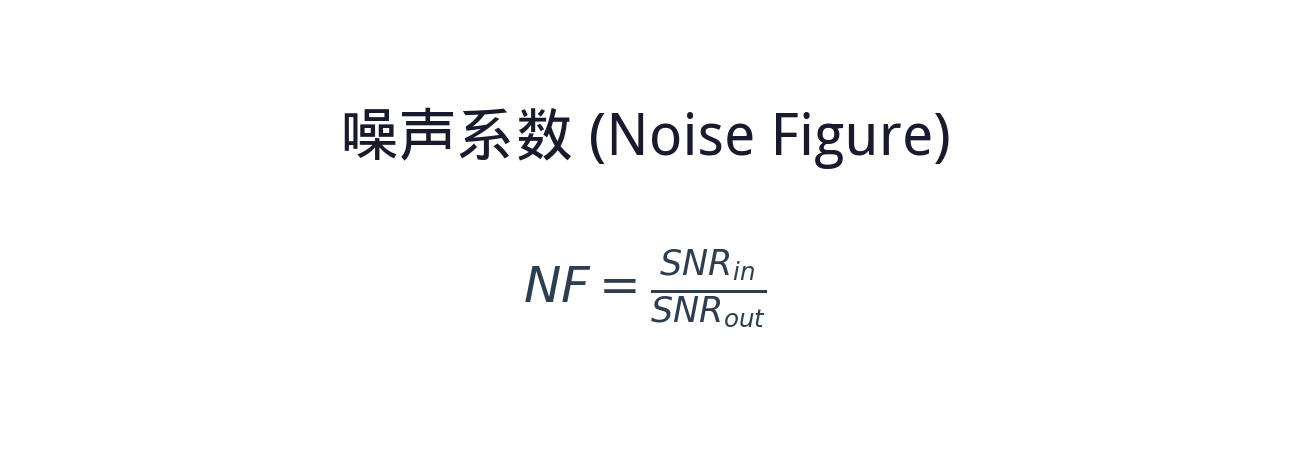
The noise figure NF is defined as the ratio of the input SNRin to the output SNRout.
The larger the NF, the more noise the amplifier adds and the more the SNR degrades.
◆ The Friis formula (cascaded noise figure)
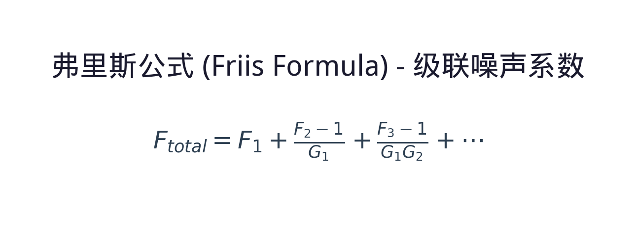
When several amplifiers are cascaded, the total noise figure is set mainly by the first stage — the noise of the first stage is amplified by every stage after it,
while the noise of the later stages is diluted by the gain ahead of them. The noise performance of the preamplifier is therefore critical.
In practice a few key parameters decide whether a device is suitable. The table below sets out the core specifications of the noise figure and what each one means:
| Parameter | Meaning | Practical significance |
|---|---|---|
| Noise figure (NF) definition | The ratio of the input SNR to the output SNR of the amplifier, in dB: NF = 10·lg(SNR_in / SNR_out), reflecting how much the amplifier degrades the signal-to-noise ratio. | The core figure for noise performance; the larger the NF, the more noise is added, the worse the output signal quality and the shorter the reach of the system. |
| Noise factor (F) | The linear-scale form of the noise figure, F = SNR_in / SNR_out, dimensionless; an ideal noiseless amplifier has F = 1, corresponding to NF = 0 dB. | The linear expression of the noise figure, widely used in analysis and derivation; the two convert into each other logarithmically. |
| 3 dB quantum limit | The theoretical minimum noise figure of a phase-insensitive amplifier at high gain, set by the quantum fluctuations of spontaneous emission and impossible to beat at any level of technology. | The physical limit for every phase-insensitive amplifier; real devices always exceed 3 dB, and those closest to it have the best noise performance. |
| Equivalent noise bandwidth | The spectral bandwidth that determines the total noise power; it depends on the gain bandwidth and on how the noise is distributed in the spectrum, and a wider bandwidth accumulates more noise power. | Directly affects the total output noise power and the SNR; the wider the bandwidth, the more noise is accumulated, which matters most for narrowband signal systems. |
| Noise figure versus temperature | Thermal noise is proportional to temperature. The noise of an optical amplifier comes mainly from spontaneous emission rather than thermal noise, but temperature changes affect the upper-level distribution and the losses of the gain medium. | Understanding the temperature dependence helps in assessing performance stability in different environments, which matters for outdoor and extreme-condition installations. |
| Cascaded noise accumulation | When several amplifiers are cascaded, the total noise figure is set mainly by the first stage (Friis formula), and the contribution of the later stages is suppressed by the gain ahead of them. | This is the core principle of multi-stage design — the first stage must be a low-noise amplifier; the accumulation rule determines the optimum architecture of the system. |
These parameters are interlinked: the noise figure trades against gain, gain trades against bandwidth, and the total noise of a cascade is almost entirely set by the first stage. No single number can therefore be used to judge an amplifier; the gain and input power at which the NF was measured matter just as much.
If some of these parameters are unfamiliar, the Soar Laser product pages carry detailed specifications, and our technical engineers can advise on selection directly.
4. Main types: what kinds of noise figure are there?
The noise figure can be classified along several dimensions, each offering a different view. Here are three: by noise source, by amplifier type and by measurement definition.
By physical origin of the noise
Spontaneous-emission noise
Caused by ASE (amplified spontaneous emission); the dominant noise source
Shot noise
The inherent noise set by the quantum nature of light
Intensity noise
Random fluctuation of the output optical power
Phase noise
Random fluctuation of the output optical phase
By typical noise figure of the amplifier type
Low-noise amplifier
A noise figure close to the quantum limit (3–4 dB), such as a good 980 nm pumped EDFA
Medium-noise amplifier
A noise figure of roughly 5–8 dB, such as a standard EDFA or a Raman amplifier
High-noise amplifier
A noise figure above 8 dB, such as a semiconductor optical amplifier
By measurement definition
Optical noise figure
A noise figure defined on the optical signal-to-noise ratio (OSNR); the definition most used for optical amplifiers
Electrical noise figure
The noise figure of the electrical signal after photodetection, which depends on the detector
Each type has its own advantages and drawbacks, and there is no absolute “best”, only what “fits”. Preamplification should use a low-noise amplifier such as a 980 nm pumped EDFA or a distributed Raman amplifier; power amplification can relax the noise requirement in exchange for more output power; and an ultra-long-haul system has to account for the accumulation of noise across the cascade.
5. Applications: where does the noise figure matter?
In engineering the noise figure is used at both ends of a project: in the link budget and in device selection. By main field it divides into the following categories:
- Optical communication system design: the noise figure sets how many amplifiers a link can carry and how far it reaches. In long-haul WDM systems the OSNR determines the bit error rate, and the noise figure of each amplifier directly sets how much that OSNR degrades.
- Preamplifier selection: the preamplifier ahead of the receiver has the strictest noise requirement because it directly sets the receiver sensitivity. A low-noise EDFA or a distributed Raman amplifier is normally chosen.
- Fibre sensing systems: in weak-signal detection such as distributed fibre sensing, the noise figure of the optical preamplifier directly sets the detection limit and the dynamic range.
- Quantum optics experiments: in quantum information and quantum key distribution the noise behaviour of the amplifier is critical, and the low noise of a phase-sensitive amplifier is a distinct advantage.
- Link budget calculation: in the design of any optical link the noise figure is a key input to the link budget, used to compute the end-to-end signal-to-noise ratio.
Typical application scenarios
Scenario 1: optical communication system design
The noise figure sets how many stages a link can carry and how far it reaches. Every EDFA adds ASE to the signal, and after N stages the OSNR degrades roughly as 10·lgN, so the more stages and the higher the noise of each, the worse the SNR at the far end. A 10 Gb/s system normally needs an OSNR above 20 dB at the receiver to keep the bit error rate below 10⁻¹², and that requirement in turn fixes the span between amplifiers and the number of repeaters a link can have.
Scenario 2: preamplifier selection
The preamplifier ahead of the receiver is the most sensitive to noise figure because it directly sets the sensitivity: every 1 dB of NF improvement buys roughly 1 dB of sensitivity, which can be several kilometres of margin. By the Friis formula the noise of the first stage is amplified by all the rest while the noise of the later stages is diluted by the gain ahead, so this is the stage worth investing in — a good 980 nm pumped EDFA reaches just over 4 dB, whereas an SOA is normally above 7 dB, and the wrong choice costs several dB of link budget outright.
Scenario 3: fibre sensing systems
In distributed sensing such as BOTDR and DTS the signal is the backscattered light returning along the fibre, six or seven orders of magnitude weaker than the launched light and already close to the detector noise floor. The noise figure of the preamplifier then sets the detection limit and the dynamic range directly: 3 dB less NF is worth several kilometres of reach, or one step better in temperature or strain resolution at the same distance.
Scenario 4: quantum optics experiments
In quantum information and quantum key distribution the extra noise of an amplifier destroys the quantum state, so the noise figure has to be as low as possible. A conventional phase-insensitive amplifier is bound by the 3 dB quantum limit, whereas a phase-sensitive amplifier can in principle go below 3 dB and approach 0 dB, which is exactly what squeezed-state generation and quantum-enhanced detection require.
Scenario 5: link budget calculation
In the design of any optical link the noise figure is a key input to the link budget. The procedure is to combine the NF and gain of every amplifier into an equivalent total noise figure with the Friis formula, then to work out the OSNR at the receiver from the launch power and the signal bandwidth, and finally to compare it with the OSNR threshold of the receiver. This step often decides feasibility more than the power margin does: a link with enough power but not enough OSNR will not run either way.
◆ Want to see more real application cases involving the noise figure? Visit the application case page of Soar Laser, or contact our technical team directly for professional advice.
6. Common misconceptions
Several fairly widespread but inaccurate beliefs circulate about the noise figure, and they need to be cleared up one by one:
Misconception 1: the noise figure is the noise power the amplifier generates
The noise figure is not an absolute noise power but the degradation of the signal-to-noise ratio. It is a ratio, dimensionless or expressed in dB, describing how much worse the SNR becomes after amplification. For the same noise figure, a higher gain also means a higher absolute output noise power.
Misconception 2: with good enough technology the noise figure can be brought down to 0 dB
It cannot. Quantum optics shows that a phase-insensitive amplifier has a theoretical lower limit of 3 dB, set by basic quantum mechanics rather than by engineering skill. Real amplifiers always sit above 3 dB because of losses and imperfections.
Misconception 3: the higher the gain, the higher the noise figure
Not necessarily. Noise figure and gain are independent parameters. Over a certain range more gain actually improves the noise figure, because the effect of input losses becomes relatively smaller; but excessive gain lets ASE saturate the amplifier and makes the noise figure worse again. The noise figure is lowest at the optimum design point.
Misconception 4: all optical amplifiers have much the same noise figure
The differences are large. A good EDFA can approach 4 dB, whereas a semiconductor optical amplifier normally sits at 6–10 dB. A distributed Raman amplifier can show a very low noise figure (even effectively negative) because it provides gain while the signal is still travelling, avoiding the degradation that comes from decaying first and being amplified afterwards. The noise figure deserves close attention at selection.
The misconceptions about the noise figure go well beyond these. New pumping schemes, low-loss coupling structures and filtering techniques keep improving, so earlier rules of thumb may no longer hold. If you have other questions, leave a comment and we will answer them one by one.
◆ Recommended reading
- What Is ASE? Where the Noise Light in an Amplifier Comes From
- What Is an EDFA? The Signal Refuelling Station of Fibre Communication
- What Is Gain? How the Amplification Capability of an Optical Amplifier Is Measured
- What Is an Optical Amplifier? Amplifying a Weak Optical Signal Directly
- What Is a Raman Amplifier? The Optical Amplifier That Uses a Scattering Effect
Leave a Reply