


I. Overview
Laser pulse-width measurement is an important concept and technique in the laser field. This article systematically introduces the relevant knowledge from the perspectives of principles, parameters, types and applications.
Ultrafast lasers — femtosecond and picosecond ultrashort pulses — are one of the “coolest” branches of laser technology. How short is a femtosecond? 1 femtosecond = 10⁻¹⁵ second; in 1 fs light travels only 0.3 micrometres — roughly a few tens of times smaller than a bacterium.
But here is the problem: how do you measure the width of a pulse this short? Ordinary photodetectors respond at best in a few tens of picoseconds, and oscilloscopes have bandwidths of a few hundred GHz — corresponding to a time resolution of a few picoseconds. Faced with a femtosecond pulse, these instruments simply “cannot see it clearly,” just as a camera with a 1-second shutter photographing a bullet passing through an apple would capture only a blur.
So measuring ultrashort pulse widths requires special “faster-than-fast” methods — the core idea is to have the pulse compare with itself, using optical methods to convert time information into spatial or intensity information, thus avoiding the speed limits of electronic devices.
A classic analogy: you want to know how fast a bullet travels but have no high-speed camera. What do you do? Fire two bullets at the same target from different distances and look at how well the bullet holes coincide — the better they overlap, the smaller the arrival-time difference. The idea behind pulse autocorrelation measurement is much the same.
The main methods of pulse-width measurement:
– Direct detection (oscilloscope + fast detector) — suitable for nanoseconds to hundreds of picoseconds
– Autocorrelator — the classic femtosecond measurement method
– FROG (Frequency-Resolved Optical Gating) — measures intensity and phase together
– SPIDER (Spectral Phase Interferometry for Direct Electric-field Reconstruction) — another phase-measurement method
– GRENOUILLE — a simplified version of FROG, cheaper and easier to use
– Streak Camera — converts time into space
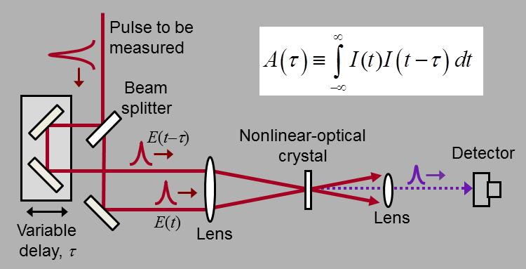
Optical-path schematic of an autocorrelator measurement setup
II. Core Principles: Main Methods for Ultrafast Pulse Measurement
1. Direct Detection (Photodetector + Oscilloscope)
This is the most direct method. Although limited in speed, it is the first choice in the nanosecond and long-picosecond regimes.
Principle: The laser pulse strikes a fast photodetector, generating an electrical pulse, which is then recorded by a high-speed oscilloscope.
Measurement range:
– Ordinary detector + oscilloscope: ~100 ps to microseconds
– Fast photodiode + 50 GHz oscilloscope: from ~10 ps
– Fastest can reach a few picoseconds (limit set by detector and oscilloscope bandwidth)
Advantages:
– Direct method, intuitive results
– Can measure pulse shape (not just width)
– Versatile equipment
Disadvantages:
– Limited speed; cannot measure femtosecond pulses
– Higher bandwidth means higher cost
– System bandwidth “broadens” the measurement, requiring deconvolution correction
The empirical relation between bandwidth and rise time:
t_r × BW ≈ 0.35. That is, if your system bandwidth is 10 GHz, the rise time is about 35 ps. To measure a 10 ps pulse you need at least 35 GHz of bandwidth.
2. Autocorrelator
The autocorrelator is the classic tool for femtosecond pulse measurement; nearly every ultrafast lab has one.
Basic principle:
- Split the pulse to be measured into two beams with a beamsplitter
- Make one beam travel a slightly longer path (adjusting the path difference with a delay line)
- Send both beams together into a nonlinear crystal (such as BBO), generating second harmonic (frequency doubling)
- The intensity of the frequency-doubled signal depends on how much the two beams overlap in time
Core formula:
I_AC(τ) = ∫ I(t) × I(t-τ) dt
where τ is the time delay between the two beams and I(t) is the pulse intensity.
Measurement process:
– When the two beams do not overlap at all → almost no frequency-doubled signal
– As the two beams begin to overlap → the frequency-doubled signal gradually strengthens
– When the two beams fully coincide → the frequency-doubled signal reaches its maximum
– Scan the delay line and record the frequency-doubled signal versus delay to obtain the autocorrelation trace
Calculating pulse width from the autocorrelation trace:
The width of the autocorrelation trace has a fixed ratio to the original pulse width, and this ratio depends on the pulse shape:
– Gaussian pulse: autocorrelation width / pulse width = √2 ≈ 1.414
– Sech² (hyperbolic-secant) pulse: ratio ≈ 1.543
– Lorentzian pulse: ratio = 2
So you must first assume the pulse shape, then use the corresponding conversion factor to turn the autocorrelation width into the pulse width. This is the autocorrelator’s biggest limitation.
Measurement range:
– Typical range: tens of femtoseconds to tens of picoseconds
– Ultrashort pulses (<10 fs): require special designs (such as zero-dispersion delay lines)
– Long pulses (>100 ps): require very long delay lines
Advantages:
– Simple principle, mature technology
– Can measure ultrashort pulses down to the femtosecond level
– Relatively inexpensive
Disadvantages:
– Measures only pulse width, not pulse shape (shape must be assumed)
– Cannot measure pulse phase (chirp information is lost)
– Scanning measurement is relatively slow
3. FROG (Frequency-Resolved Optical Gating)
FROG was invented by Professor Rick Trebino’s team in 1991; it solved the autocorrelator’s inability to measure phase.
Basic principle: FROG combines autocorrelation with spectral measurement. Instead of measuring only the total intensity of the frequency-doubled signal, it uses a spectrometer to measure the frequency-doubled spectrum at each delay — producing a two-dimensional plot (the FROG trace) with wavelength on the horizontal axis and time delay on the vertical axis.
From this two-dimensional plot, an iterative algorithm (such as principal-component generalized projections, PCGP) can completely reconstruct the pulse’s electric field — including amplitude and phase. In other words, FROG tells you not only the pulse width, but also whether the pulse is chirped and how the phase is distributed.
Types of FROG:
– SHG-FROG: most common, based on second-harmonic generation, high sensitivity
– PG-FROG: based on polarisation gating, suitable for very broad spectra
– TG-FROG: based on transient grating
– XFROG: uses a known reference pulse for cross-correlation
Advantages:
– Completely reconstructs pulse amplitude and phase
– No need to assume the pulse shape
– Rich information; can diagnose pulse quality
Disadvantages:
– Fairly complex algorithms
– More expensive than autocorrelators
– Measurement and reconstruction take some time
4. SPIDER (Spectral Phase Interferometry for Direct Electric-field Reconstruction)
SPIDER is another phase-measurement technique, invented by Professor Ian Walmsley’s team.
Basic principle: The pulse under test is mixed with two spectrally sheared replicas (with a frequency difference produced by chirping) via sum-frequency generation, yielding two spectrally sheared signals. By measuring the interference spectrum of these two signals, the spectral phase of the pulse can be extracted directly.
Unlike FROG, SPIDER does not require an iterative algorithm — the phase can be calculated directly from the spectrum, making it very fast.
Advantages:
– Fast reconstruction (no iteration)
– High accuracy
– Also works for very broad spectra
Disadvantages:
– Fairly complex optical setup
– Requires precise control of the chirped pulses
– Demanding on environmental stability
5. GRENOUILLE (Grating-Eliminated No-nonsense Observation of Ultrafast Incident Laser Light E-field)
GRENOUILLE can be understood as a “simplified version” of FROG, also invented by Trebino’s team. The name is interesting — it means “frog” in French, echoing FROG (frog).
Basic principle: It uses a cylindrical lens and a Fresnel biprism in place of the delay line and spectrometer grating in a traditional FROG, greatly simplifying the structure. It maps both delay and wavelength onto spatial positions, so a single CCD camera exposure captures the complete FROG trace.
Advantages:
– Simple structure, no moving parts
– Relatively inexpensive
– Easy to use, low alignment requirements
Disadvantages:
– Limited range of measurable pulse widths
– Slightly lower accuracy than traditional FROG
– Best suited to teaching and routine measurements
6. Streak Camera
The streak camera is another ultrafast measurement tool; it converts time information into spatial information.
Principle: A light pulse strikes a photocathode, producing photoelectrons. These electrons pass through a fast deflection field (the deflection voltage changes rapidly with time); electrons arriving at different times are deflected by different amounts and land at different positions on a phosphor screen — time is “stretched” into a spatial distribution.
Temporal resolution: The best streak cameras can reach a few hundred femtoseconds.
Advantages:
– A single measurement gives the complete pulse shape
– Can be combined with a spectrometer (time-resolved spectroscopy)
– Suitable for extremely weak light and fluorescence measurements
Disadvantages:
– Very expensive (hundreds of thousands to over a million)
– Complex maintenance (requires high-voltage supply and vacuum system)
– Temporal resolution inferior to autocorrelation/FROG (fastest a few hundred femtoseconds)
III. Accuracy Comparison of the Methods
| Measurement method | Temporal resolution | Measures phase? | Pulse shape | Price level | Applicable range |
|---|---|---|---|---|---|
| Direct detection | ~5 ps | No | Yes | Low → medium | nanoseconds to long picoseconds |
| Autocorrelator | ~5 fs | No | Must assume | Medium | femtoseconds to tens of picoseconds |
| FROG | ~5 fs | Yes | Yes | Medium → high | femtoseconds to tens of picoseconds |
| SPIDER | ~5 fs | Yes | Yes | High | femtoseconds to a few picoseconds |
| GRENOUILLE | ~20 fs | Yes | Yes | Medium | tens of femtoseconds to a few picoseconds |
| Streak camera | ~100 fs | No | Yes | High | hundreds of femtoseconds to nanoseconds |
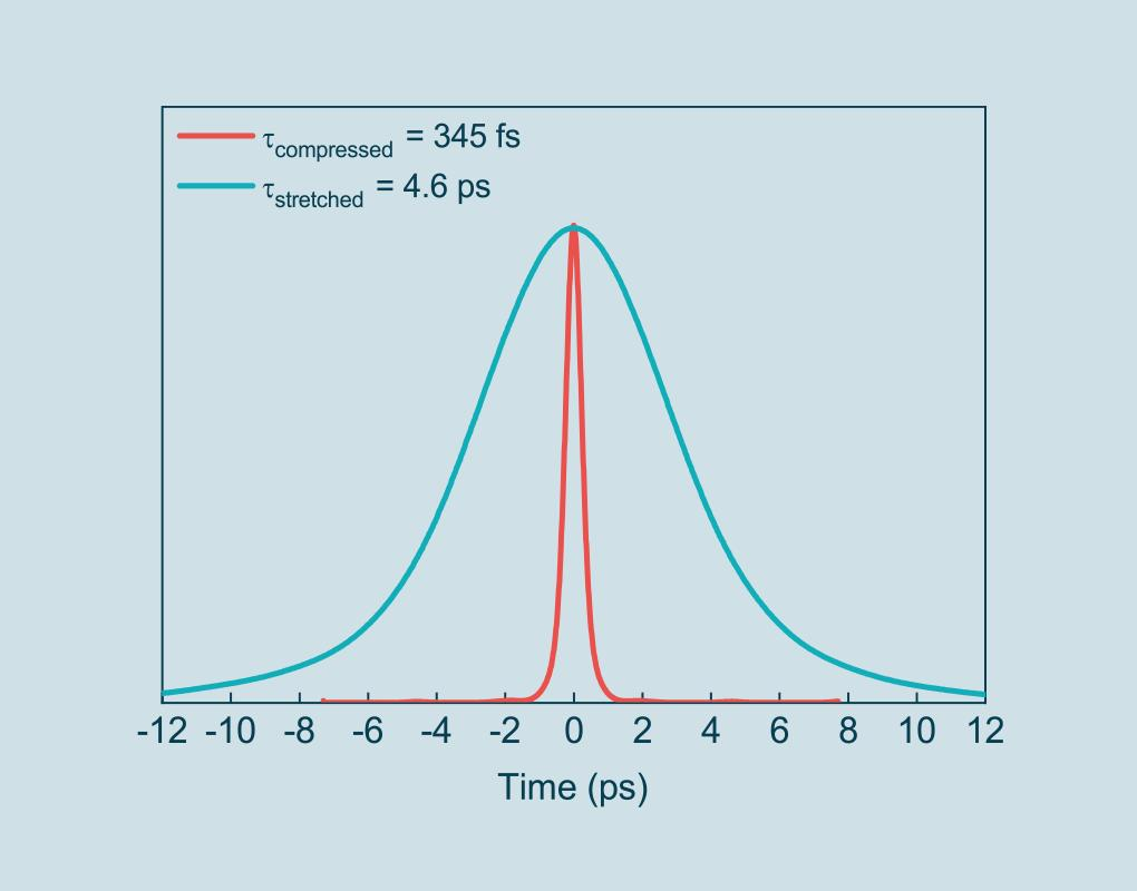
Time-domain comparison of compressed and stretched pulses
IV. Common Misconceptions
Misconception 1: An autocorrelator directly measures the pulse width
No. An autocorrelator measures the width of the autocorrelation function, not the pulse width. You must first assume the pulse shape (Gaussian? sech²?) and then use the corresponding conversion factor.
What is more troublesome: if the pulse shape is complex (for example with pedestals or side lobes), the autocorrelation result can be seriously distorted. Because autocorrelation is an “averaging” process that smooths over complex structure. This is why research tends to prefer FROG over a simple autocorrelator.
Misconception 2: Shorter pulses are always better; femtosecond is necessarily superior to picosecond
Pulse width is only one parameter of a pulse; whether shorter is better depends on the application:
– For micromachining → pulse energy and repetition rate may matter more, and pulse widths in the picosecond-to-nanosecond range can be more appropriate
– For multiphoton imaging → femtosecond pulses do have advantages (high peak power)
– For spectroscopy → short pulses correspond to broad spectra, which may have unwanted side effects
Moreover, the shorter the pulse, the more demanding the dispersion control — a little dispersion broadens the pulse. Short-pulse lasers are also more complex to maintain and use.
Misconception 3: A pulse reconstructed by FROG is necessarily accurate
FROG is indeed powerful, but it has limitations:
– FROG reconstruction has “ambiguities” — for example ambiguity in the time direction, where you cannot tell whether the pulse was strong-then-weak or weak-then-strong
– The reconstruction algorithm is iterative and may converge to a local optimum with poor initial values
– Measurement noise affects the reconstruction result
– Some extremely complex pulse shapes may not reconstruct well
So FROG results should also be judged with common sense and not blindly trusted.
Misconception 4: All ultrafast pulse-measurement instruments can be used casually
Ultrafast measurement equipment is “delicate”; improper use gives inaccurate results or no result at all:
– Dispersion: optical components inside an autocorrelator introduce dispersion and broaden the pulse, especially when measuring ultrashort pulses below 10 fs, where dispersion compensation is mandatory
– Alignment: the two beams must overlap strictly in space inside the nonlinear crystal, otherwise frequency-doubling efficiency is low and the signal weak and inaccurate
– Power: too low a power gives a weak signal; too high a power damages the crystal and may produce higher-order nonlinear effects
– Polarisation: frequency doubling is polarisation-sensitive; the input polarisation must match the crystal
V. Selection Advice
1. Select by Measurement Needs
- Only need a rough idea of the pulse width, pulse shape unimportant → autocorrelator, the best value for money
- Need complete pulse information (intensity + phase) for research → FROG or SPIDER
- Teaching lab, limited budget → GRENOUILLE or an entry-level autocorrelator
- Measuring long pulses (hundreds of picoseconds to nanoseconds) → fast detector + oscilloscope
- Measuring extremely weak light or fluorescence lifetime → streak camera or time-correlated single-photon counting (TCSPC)
2. Key Parameters
- Measurement range: does the measurable pulse-width range cover your needs
- Wavelength range: does it suit your laser wavelength
- Sensitivity: the minimum pulse energy needed for a measurement
- Measurement speed: scanning types are slow, single-shot types are fast
- Software features: support for multiple pulse-shape fits, FROG reconstruction, etc.
3. Practical Advice
- When buying an autocorrelator, confirm which pulse-shape fits are included (Gaussian, sech², Lorentzian, etc.)
- When buying a FROG, check whether the reconstruction algorithm is mature and whether technical support is available
- If measuring very short pulses (<30 fs), be sure to confirm the instrument’s dispersion-compensation capability
- Consider whether you need a fibre-coupled version (more convenient to use, but introduces extra dispersion)
VI. Application Scenarios
1. Ultrafast Laser R&D
- Mode-locked laser pulse-width monitoring and optimisation
- Debugging of pulse-compression systems
- Quality inspection of amplifier output pulses
- Verification of dispersion management
2. Ultrafast Spectroscopy
- Pump-probe experiments
- Transient absorption spectroscopy
- Time-resolved fluorescence
- Chemical reaction dynamics research
3. Laser Micromachining
- Quality control of ultrafast laser processing equipment
- Optimisation of processing parameters
- Pulse stability monitoring
4. Biomedical Imaging
- Pulse quality inspection of multiphoton microscopes
- Characterisation of OCT (optical coherence tomography) light sources
- Parameter monitoring of femtosecond laser surgery
5. Communications and Information Processing
- Pulse characterisation for high-speed optical communication
- Optical soliton propagation research
- All-optical signal processing
VII. Recommended Reading
- What Is an Autocorrelator? How to Measure Ultrashort Pulse Width
- What Is FROG? How to Measure Pulse Intensity and Phase Together
- What Is Mode Locking? How to Obtain Femtosecond Ultrafast Pulses
- What Is Q-Switching? How to Generate High-Energy Pulsed Lasers
- What Is a Photodetector? How Light Signals Become Electrical Signals
- What Is a Photodiode? The Most Basic Photodetector
References: Principles and Technology of Ultrafast Lasers, RP Photonics Encyclopedia – Ultrashort Pulses, R. Trebino, Frequency-Resolved Optical Gating: The Measurement of Ultrashort Laser Pulses
Leave a Reply