


I. Overview
Optical resolution and imaging quality evaluation is an important concept and technology in the laser field. This article systematically introduces the relevant knowledge from the perspectives of principles, parameters, types and applications.
When buying a camera lens, you may look at the “resolution” figure — how many line pairs per millimetre (lp/mm). When building a microscope system, you care about the “resolution limit” — how small a detail you can resolve. When designing a projection lens, you use the MTF curve to assess image quality.
Resolution and imaging quality are the core metrics of every optical imaging system. Whether it is a camera, microscope, telescope, lithography tool or laser processing head, the final performance depends to a great extent on imaging quality.
But did you know? The word “resolution” is actually quite vague. Two people saying “high resolution” may mean completely different things. One may mean the smallest resolvable detail, another the pixel count, and yet another the contrast. To evaluate an optical system’s imaging quality scientifically, a complete set of theories and methods is needed — from the Rayleigh criterion to MTF, from PSF to OTF, each concept has its own specific meaning and use.
An interesting historical story: in the 19th century, astronomers debated how close two stars a telescope could actually resolve. Lord Rayleigh proposed a criterion in 1879 — when the centre of one star’s Airy disk falls exactly on the first dark ring of the other’s, the two stars are just resolvable. This is the famous “Rayleigh criterion,” which remains the classic standard for evaluating resolution to this day.
The main methods for evaluating imaging quality:
– Resolution and the Rayleigh criterion (the most basic concept)
– Point spread function PSF (complete description in the spatial domain)
– Modulation transfer function MTF (quantitative evaluation in the frequency domain)
– Optical transfer function OTF (complete description of amplitude + phase)
– Aberration analysis (wavefront aberration, Seidel aberrations, etc.)
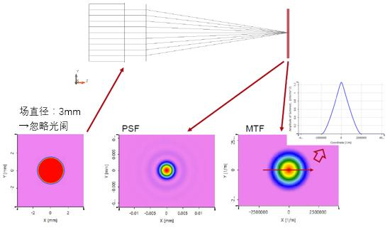
Schematic of the relationship between an optical system’s PSF and MTF
II. Core Principles
1. Resolution and the Rayleigh Criterion
What is resolution?
Resolution, quite simply, is the ability of an optical system to distinguish two closely spaced objects. The closer two points can be while still being seen as two separate points, the higher the resolution.
But why is there a resolution limit? Because light has wave nature — an ideal point source, after passing through an optical system, does not focus to an ideal point but forms a diffraction spot (an Airy disk).
Size of the Airy disk:
d = 2.44 × λ × f / D = 2.44 × λ × F/#
where:
– λ is the wavelength
– f is the focal length
– D is the aperture diameter
– F/# is the f-number (f/D)
The Rayleigh Criterion
The Rayleigh criterion states: when the centre of one point source’s Airy disk falls exactly on the first dark ring of another point source’s Airy disk, the two points are just resolvable.
The angular separation between the two points at this moment is:
θ = 1.22 × λ / D (angle, in radians)
The corresponding linear distance (in the image plane):
δ = 0.61 × λ / NA
where NA is the numerical aperture, NA = n × sin θ, and n is the refractive index of the medium.
Other Criteria
The Rayleigh criterion is not the only standard:
– Sparrow Criterion: stricter than Rayleigh, the limit is when the dip between two Airy disks just disappears
– Dawes’ Limit: an empirical criterion commonly used in astronomy, slightly more lenient than the Rayleigh criterion
– 100% contrast criterion: the two points are completely separated (valley value of 0)
Why are there different criteria? Because “just resolvable” is itself a subjective concept — some people have sharper eyes and can see finer differences; others cannot. Hence the need for various objective standards to unify the wording.
2. Point Spread Function PSF (Point Spread Function)
What is the PSF? The intensity distribution formed in the image plane when an ideal point source passes through an optical system is called the point spread function.
You can think of the PSF as the “fingerprint” of an optical system — every system has its own unique PSF. If the system is ideal (diffraction only, no aberrations), the PSF is the Airy disk; if the system has aberrations, the PSF becomes more complex and more diffuse.
Importance of the PSF:
– The PSF completely describes the imaging characteristics of the optical system (spatial domain)
– The image of any object = the convolution of the object with the PSF
– The narrower and sharper the PSF, the clearer the system’s image
Strehl Ratio:
The Strehl ratio is a concise index for evaluating imaging quality. It equals peak intensity of the aberrated system’s PSF / peak intensity of the aberration-free (diffraction-limited) system’s PSF.
- Strehl ratio > 0.8: generally considered “diffraction-limited” class (an approximation of the Rayleigh quarter-wave criterion)
- 0.5 < Strehl ratio < 0.8: moderate aberrations
- < 0.5: severe aberrations
3. Modulation Transfer Function MTF (Modulation Transfer Function)
MTF is currently the most widely used and most comprehensive method for evaluating imaging quality.
What is MTF?
Imagine using an optical system to look at a set of sinusoidal fringes (alternating bright and dark lines):
– If the fringes are coarse (low spatial frequency), the system reproduces them well and contrast is high
– If the fringes are fine (high spatial frequency), the reproduced contrast decreases
– When the fringes are fine enough that contrast drops to 0, the system cannot resolve them at all
MTF is the curve of contrast as a function of spatial frequency. It describes an optical system’s ability to transfer detail of different fineness.
Definition of MTF:
MTF(f) = image modulation / object modulation
Modulation (contrast) = (maximum intensity – minimum intensity) / (maximum intensity + minimum intensity)
How to read an MTF curve?
There are several key points when reading an MTF curve:
1. Low-frequency end (<10 lp/mm): reflects the contrast of large-scale detail, related to “transparency”
2. Mid-frequency range: reflects overall sharpness
3. Cutoff frequency: the spatial frequency at which MTF drops to 0, corresponding to the resolution limit
4. Area under the MTF curve: roughly reflects overall imaging quality
Diffraction-Limited MTF
An ideal aberration-free optical system still does not have an MTF that is a flat line at 100% — because of diffraction, the MTF gradually falls from 1 (low frequency) to 0 (cutoff frequency).
Diffraction-limited cutoff frequency:
f_c = 1 / (λ × F/#) = 2NA / λ
The Relationship Between MTF and PSF
PSF and MTF are a Fourier transform pair:
– MTF is the modulus of the Fourier transform of the PSF
– In other words, the point spread function in the spatial domain becomes the optical transfer function in the frequency domain
This gives us two equivalent ways to describe imaging quality:
– Spatial domain (PSF): intuitive, you can see the actual spot shape
– Frequency domain (MTF/OTF): quantitative, easy to compare the performance of different systems
4. Optical Transfer Function OTF (Optical Transfer Function)
OTF is more complete than MTF — MTF only describes changes in amplitude (contrast), while OTF also includes phase information.
OTF(f) = MTF(f) × e^{i×PTF(f)}
where PTF is the phase transfer function.
Why is phase needed? Because phase changes affect the position and symmetry of the image. If the PTF is linear, it only causes an overall shift of the image (no problem); but if the PTF is nonlinear, it causes distortion and asymmetry of the image.
In most imaging applications MTF is sufficient (because the human eye and detectors are insensitive to phase). But in some special applications (such as phase imaging and interferometry), the PTF also matters.
5. Aberrations: The Cause of Degraded Imaging Quality
Why do real optical systems fail to reach the diffraction limit? Because of aberrations.
The main monochromatic aberrations (Seidel aberrations):
– Spherical aberration: for on-axis points, rays at different heights focus at different positions
– Coma: for off-axis points, the image trails like a comet’s tail
– Astigmatism: for off-axis points, the sagittal and tangential directions focus at different positions
– Field curvature: the image surface is curved rather than flat
– Distortion: geometric deformation of the image (pincushion, barrel)
Chromatic aberration:
– Axial chromatic aberration: different wavelengths focus at different positions
– Lateral chromatic aberration: different wavelengths have different magnifications
Aberrations enlarge and deform the PSF and lower the MTF. One of the core tasks of optical design is to correct aberrations by properly choosing lens materials, curvatures, spacings and so on.
III. Key Parameters and Metrics
| Parameter | Meaning | Unit |
|---|---|---|
| Resolution | smallest resolvable detail | The ability of an optical system to distinguish two adjacent object points; the most core performance metric of an imaging system, determining how clear the image is. |
| NA (Numerical Aperture) | light-gathering ability | Determines the system’s light-gathering ability and resolution limit; higher NA means better resolution, and it is one of the most important parameters of an objective lens. |
| F/# (f-number) | relative aperture | The ratio of focal length to clear aperture, corresponding to NA; affects image brightness, depth of field and resolution. |
| Strehl Ratio | peak intensity ratio | The ratio of the actual image point’s peak intensity to the ideal Airy disk’s peak intensity, comprehensively reflecting the effect of aberrations on imaging quality. |
| MTF cutoff frequency | frequency at which MTF falls to zero | The spatial frequency at which the modulation transfer function drops to zero; the frequency-domain representation of the system’s resolution limit. |
| MTF@a given frequency | contrast at a specified frequency | The modulation transfer function value at a specific spatial frequency, reflecting the system’s ability to transfer detail at that frequency. |
| Wavefront error RMS | root-mean-square wavefront error | The root-mean-square value of wavefront error, a quantitative index for evaluating an imaging system’s aberration level, usually expressed in units of wavelength. |
| Rayleigh-criterion resolution | smallest resolvable size under the Rayleigh criterion | The resolution limit based on the Rayleigh criterion, the most classic definition of resolution, convenient for comparing different systems. |
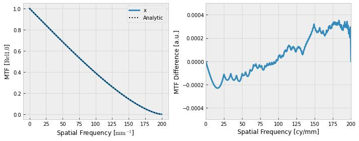
Example MTF curve of the modulation transfer function
IV. Common Misconceptions
Misconception 1: The more pixels, the higher the resolution
This is the most common misconception. Many people think “pixel count = resolution,” but that is not the case. An optical system’s resolution is determined by the optical lens, while pixels are a detector parameter. The relationship between the two is like a faucet and a pipe — the lens is the faucet (determining the maximum flow), the pixels are the pipe (determining how much you can catch). If the lens itself can only resolve 100 lp/mm, using a detector that resolves 1000 lp/mm is useless; the extra pixels merely sample a blurred image.
The correct approach is: match the optical resolution to the detector pixels. The common design rule is “2–3 pixels per Airy disk” (a Nyquist-sampling consideration).
Misconception 2: High resolution means good imaging quality
Resolution is only one aspect of imaging quality. Two systems may have the same cutoff frequency but very different MTF curves:
– One system may have very high low-frequency contrast but an ordinary cutoff frequency
– Another may have a very high cutoff frequency but poor low- and mid-frequency contrast
In actual visual impression, the first system may look more “transparent” and sharper; although the second can show finer lines, its low contrast makes it look “grayish.” So evaluating imaging quality requires looking at the full MTF curve, not just a single resolution number.
Misconception 3: The Rayleigh criterion is the absolute resolution limit
The Rayleigh criterion is only a “conventional” standard, not a physical law. In reality:
– If the signal-to-noise ratio is high enough, you can resolve two points closer than the Rayleigh limit (super-resolution)
– Modern image-processing techniques (such as deconvolution and deep learning) can recover higher-resolution information from data below the diffraction limit
– The Sparrow criterion is stricter than the Rayleigh criterion (can resolve closer points)
The value of the Rayleigh criterion is that it provides a convenient, reproducible comparison standard — not that “beyond this limit is absolutely impossible.”
Misconception 4: The higher the MTF curve, the better, and the lens you buy matches the specification
MTF quoted values are usually “design values” or “best-case values”; in actual use MTF is affected by many factors:
– Aperture: the smaller the F/# (larger aperture), the larger the aberrations usually are and the lower the MTF
– Field position: MTF is highest at the centre and falls toward the edge
– Wavelength: MTF differs with wavelength, and chromatic aberration lowers MTF
– Focus: poor focus seriously reduces MTF
– Manufacturing tolerance: real products always deviate from the design value
So when looking at an MTF curve, pay attention to the conditions under which it was measured — centre or edge? Best aperture or widest aperture? Single wavelength or full spectrum?
V. Selection Advice
1. Select the Evaluation Method by Application
- Simply comparing lens quality → look at the MTF curve (most intuitive)
- Microscope system design → look at NA and resolution (Rayleigh criterion)
- High-precision imaging systems → look at Strehl ratio and wavefront aberration
- When a complete evaluation is needed → use PSF + MTF + aberration analysis in combination
- Subjective evaluation of image quality → combine with actual capture results
2. Optical System Selection Points
- Need high resolution? → choose a system with large NA and small F/#
- Need high contrast? → pay attention to chromatic-aberration correction and stray-light control
- Large-field imaging? → focus on the MTF and distortion at the field edge
- Broad-spectrum applications? → pay attention to chromatic-aberration correction; choose an apochromatic design
- Low-light imaging? → large aperture (small F/#) + high transmittance
3. Imaging Quality Test Equipment
- MTF tester: directly measures the MTF curve, suitable for production-line QC and lens evaluation
- Interferometer: measures wavefront aberration with high precision, suitable for high-precision optical systems
- Resolution target: tested with a standard resolution chart, simple and intuitive
- Knife-edge tester: measures the edge spread function of the PSF, a classic method
VI. Application Scenarios
1. Photography and Videography
- Evaluation and comparison of lens imaging quality
- Camera sensor and lens matching design
- Image quality testing and optimisation
2. Microscopy and Life Sciences
- NA and resolution specifications of microscope objectives
- Imaging quality assessment of fluorescence and confocal microscopes
- Resolution characterisation of super-resolution microscopes (STED, PALM/STORM)
3. Semiconductor Lithography
- Lithography lenses are among the most precise optical systems in the world
- Resolution directly determines the chip process node
- EUV lithography resolution reaches the few-nanometre level
4. Laser Processing
- Focused spot size directly affects processing precision
- Beam quality and focusing optics together determine processing resolution
- High-power laser processing must also consider changes in “effective resolution” caused by thermal effects
5. Astronomical Observation
- Telescope resolution is limited by both the diffraction limit and atmospheric turbulence
- Adaptive optics can partially compensate for atmospheric disturbance, approaching the diffraction limit
- The main goal of large-aperture telescopes is to improve resolution and light-gathering ability
6. Optical Design and Manufacturing
- Imaging quality simulation during lens design
- Quality inspection of optical components after fabrication
- Performance testing and calibration after lens assembly
VII. Recommended Reading
- What Is Beam Quality? Why Some Lasers Can Focus to a Smaller Spot
- The M² Factor Explained: The International Standard Measure of Beam Quality
- What Is a Wavefront? Why It Is Called the Contour Map of a Laser
- What Is a Beam Profile? The Intensity Distribution Across a Laser’s Cross-Section
- Laser Beam Quality Analyser
- Optical Resonators and Optical Components
References: Principles of Optics (Born & Wolf), Engineering Optics, Modern Optical Engineering (W. Smith), RP Photonics Encyclopedia – Resolution
Leave a Reply